Apache Paimon: one table for the stream and the report

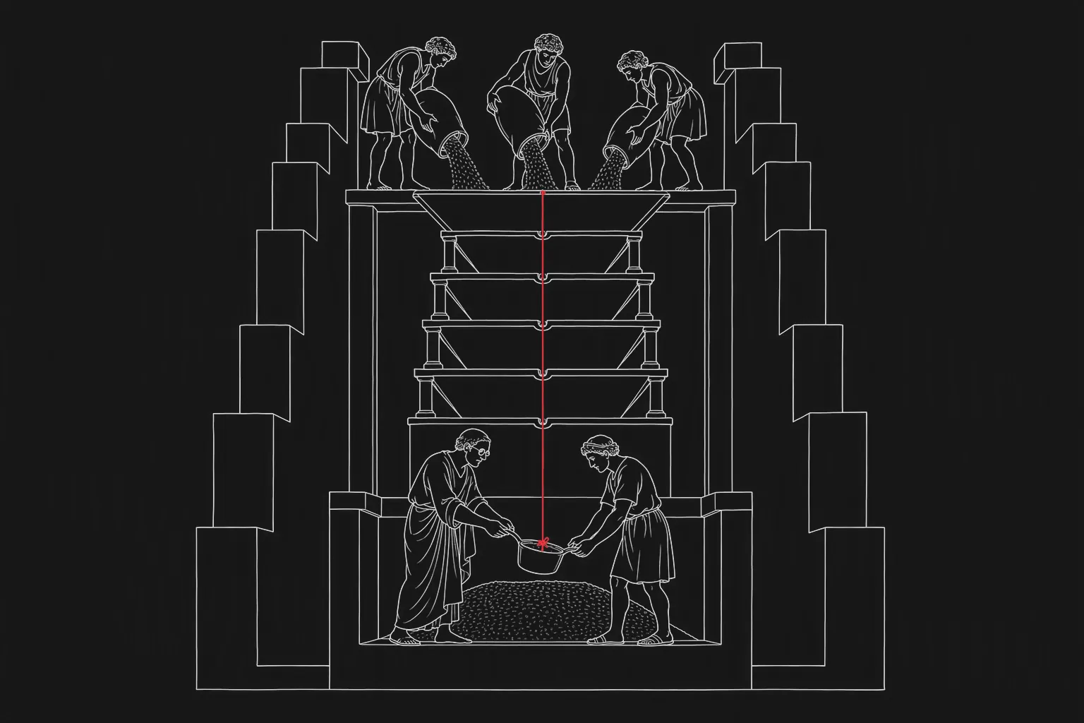
A serial manufacturer keeps the state of a production order in three places. The MES knows which operation is running and how many pieces have passed. The ERP knows the quantity ordered, the due date and the customer. The quality system knows the rejects. The planner opens all three every morning and writes the real state into a spreadsheet, because no single system has it.

An AI-native planning assistant cannot work from that spreadsheet, and it should not open three systems either. It needs one table in which the order state is already assembled and stays current as the shop floor moves. Among the open table formats, Apache Paimon is the one designed with that table in mind. Where it sits in the two memories of an enterprise system is the subject of this profile; how an agent reads such a table is covered separately in the state your agents act on.

Why a continuously updated table is hard

Table formats built for batch loads store data in immutable Parquet files and describe them with metadata. Updating one row means writing a new file and marking the old one, or recording a deletion against it. At a few updates a minute that is fine. At a stream of MES events, every micro-batch produces new files, the metadata grows, and a compaction job has to run constantly just to keep reads from opening thousands of files. The format was not wrong; it was built for a different write pattern.

Paimon starts from the write pattern. Its primary-key tables are organised as a log-structured merge-tree per bucket: incoming rows land sorted in a small top level, and compaction merges levels downwards, keeping one current version per key. Merging is part of the storage model, not a maintenance task bolted onto it. Tables without a primary key are append tables; they accept only inserts and support batch DELETE, UPDATE and MERGE INTO.

The current release is Paimon 2.0.0 of 7 August 2026, shipped together with PyPaimon 2.0.0; 1.4.2 came in June and 1.3.0 in October 2025 (checked 21 October 2026). The architecture below is from the project documentation and did not change between those versions.

The pieces that matter to an architect

Buckets and partitions. A primary-key table is split into partitions and, within each, into buckets by a hash of the key. The bucket is the unit of the LSM tree and of parallel writes. Choosing the bucket count is a sizing decision, not a default to accept.

Merge engines. This is the feature that moves business logic out of the stream job and into the table. The merge engine says what happens when a second row arrives for the same key. deduplicate, the default, keeps the latest. partial-update fills in only the columns the new row carries, so three systems can each write their columns of one order row; sequence groups decide which source wins per column group. aggregation applies a function per column — sum, max, last value. first-row keeps the first and ignores the rest. For the manufacturer, the order state table is a partial-update table: the ERP writes quantity and due date, the MES writes operation and pieces done, the quality system writes rejects, and nobody writes a join.

Changelog producers. A downstream consumer needs to know what changed, not only what is current. The changelog producer setting decides how the table emits that: none, input when the stream already carries complete change records, lookup when the table has to compute before-and-after images itself at write time, full-compaction when it is acceptable to emit them at each full compaction. The choice trades write latency against cost; it belongs in the specification.

Snapshots and tags. Every commit creates a snapshot; snapshots expire on a schedule. A tag pins a snapshot’s files so that a state — end of shift, end of month, the moment a planning decision was made — can be read back after the surrounding snapshots are gone.

Engines. The engine matrix lists Flink and Spark for reading and writing, Hive, Trino and Presto for queries, and StarRocks and Doris for reads. Flink is the engine the format grew up with, and streaming writes in practice mean Flink.

Infographic

Inside a Paimon primary-key table

1. 01Incoming eventsRows from the ERP, the MES and the quality system, each carrying the order key.
2. 02Level 0New versions land sorted by key in small files; the latest write is visible at once.
3. 03Compaction levelsBackground merging applies the merge engine and keeps one current row per key per level.
4. 04Snapshot and tagEach commit is a snapshot; a tag pins the state at a chosen moment.
5. 05ReadersFlink and Spark read and write; Trino, Hive, Presto, StarRocks and Doris read.

A manufacturer’s order state table

Consider a serial manufacturer with an ERP, an MES and a quality system, building one table of production-order state. This is an illustration, not a client case.

Before: the planner assembles the state by hand each morning. The operator sees the MES only. The sales desk asks the planner. A planning assistant, if it existed, would have nothing consistent to read.

With Paimon: change events from the three systems reach Kafka with registered schemas; Flink writes them into a partial-update table keyed by production order, with a sequence group per source system so that the MES cannot overwrite the ERP’s due date. The planner, the operator’s screen and the planning agent read the same table. A tag is created at the end of each shift. The agent proposes resequencing when a reject rate crosses a threshold; the planner decides, and the decision is entered in the ERP, from which it flows back into the table like every other change.

What to measure: lag from an MES event to its visibility in the table; the number of places where “order state” is held, which should fall to one; the cost of Flink and compaction per month; and the time to answer “what did the planner see at 14:00” from a tag.

Where the cost goes, and where the decisions sit

A Paimon table is never finished writing. Compaction runs as long as events arrive, and its compute is a standing cost that a batch table does not have. The lookup changelog producer adds work at write time; the full-compaction producer adds latency. A bucket count set too low limits write parallelism; set too high, it multiplies small files. These are the numbers that decide whether the one table costs less than the three it replaces.

In an AI development lifecycle the merge-engine configuration, the sequence groups, the changelog producer and the bucket count are part of the table’s specification, written before the stream job, with the person who approved each. The acceptance test is a replay: a day of events from the three systems run into a fresh table, and the result compared row by row with the state the planner had in the spreadsheet. Coding agents draft the Flink job, propose a merge configuration from the event schemas and generate the replay harness well. They should not decide which source wins a column, how long snapshots live, or whether a decision needs seconds; those are the engineer’s and the process owner’s signatures.

What a good outcome looks like

One table of order state that three roles and one agent read, with a published lag, a tag per shift, and a compaction bill that was estimated before the first event arrived. Fewer places where the state is kept, not more. And a replay test that runs before every change to the merge rules.

Our part

In AI data engineering we specify and build such tables: the event contracts, the merge engines and sequence groups, the changelog settings, the tags and the replay tests — with the compaction cost estimated up front and an owner for every setting that can change the state. We do not resell platforms. More about predictes is on the home page.